Mapa de area de estudio en R

Paquetes necesarios

library(raster)
library(leaflet)
library(sf)
library(osmdata)
library(tidyverse)
library(rworldxtra)
library(cowplot)
library(ggspatial)
library(tmap)

1. Obteniendo mapa de Colombia

data("countriesHigh")
Mundo <- st_as_sf(countriesHigh)
colombia <- Mundo %>%  select(ne_10m_adm) %>% filter(ne_10m_adm=="COL")

2. Obteniendo mapa de Santa marta

col <- getData('GADM', country='COL', level=2)
col <- st_as_sf(col)
sm <- col %>% filter(NAME_2 == "Santa Marta (Dist. Esp.)")

3. localizando punto de area de estudio

lugar <- data.frame(lon = c(-74.18637,-74.17878 ), lat = c(11.22167, 11.2266), 
                    Lugares = c("Bosque Unimag", "Quinta de San Pedro")) %>% 
        st_as_sf(coords = c(1,2), crs = "+proj=longlat +datum=WGS84")

4. Obtenemos los rios de Santa Marta

agua <- opq(bbox = 'santa marta, magdalena') %>% 
        add_osm_feature(key = 'waterway', value = "river") %>%
        osmdata_sf()
rios <- agua[["osm_lines"]] %>% st_as_sf()
rios <- rios %>% filter(!is.na(name) & name != "toribio")

5. creando un cuadro alrededor de Santa Marta

sm_box <- st_as_sfc(st_bbox(sm))

6. Descragamos los datos de altura para la zona de estudio

altura <- getData("SRTM", lon=-74.1869902, lat = 11.2206088)

7. Cortamos el raster solo para Santa Marta

raster_sm <- altura %>% crop(sm) %>% mask(sm)

8. ver el corte

plot(raster_sm, colNA = "black")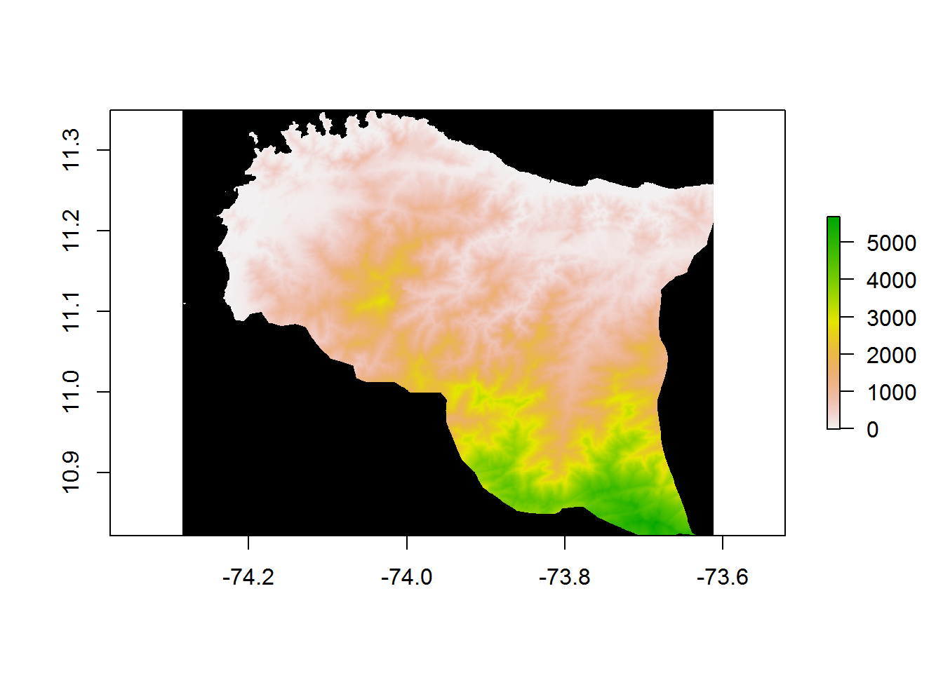

9. convertimos el raster en un DF

altura_DF <- raster_sm %>% as("SpatialPixelsDataFrame") %>% 
        as.data.frame() %>% rename(msnm =srtm_22_10) %>% mutate(Altitud = msnm/10)

10. Creamos el mapa de Colombia

mapa_1 <- mapa1 <- ggplot() + geom_sf(data = colombia, fill = "white") + 
        geom_sf(data = sm_box, fill = NA, color= "red") + 
        ggtitle("Macrolocalizacion") +
        theme_bw() + theme(panel.grid.major = element_blank(),
                           panel.grid.minor = element_blank(),
                           axis.text.x = element_blank(),
                           axis.text.y = element_blank(),
                           plot.title = element_text(hjust = 0.5, size = 7))

11. Mapa principal

#Creando paleta de colores
col <- c('#bcd2a4','#89d2a4','#28a77e','#90b262',
'#ddb747','#fecf5b','#da9248','#b75554',
'#ad7562','#b8a29a','#9f9e98')

relevo.col <- colorRampPalette(col)

mapa_2 <- ggplot()  +
        geom_tile(data = altura_DF, aes(x=x,y=y,fill= Altitud)) +
        geom_sf(data = rios, color ="blue") + 
        geom_sf(data = lugar, aes(color = Lugares)) + 
        annotation_north_arrow(location ="tr",
                               which_north ="true",
                               style = north_arrow_fancy_orienteering()) +
        annotation_scale(location = "br") + 
        scale_fill_gradientn(colours = relevo.col(40), na.value = "trasparent") + 
        scale_color_manual(values = c("red", "yellow")) +  theme_bw() + xlab(NULL) + ylab(NULL)

12. Uniendo los mapas

mapa_final <- ggdraw() + 
        draw_plot(mapa_2) +
        draw_plot(mapa_1, x=0.05, y= 0.17, width=0.3, height=0.28)


mapa_final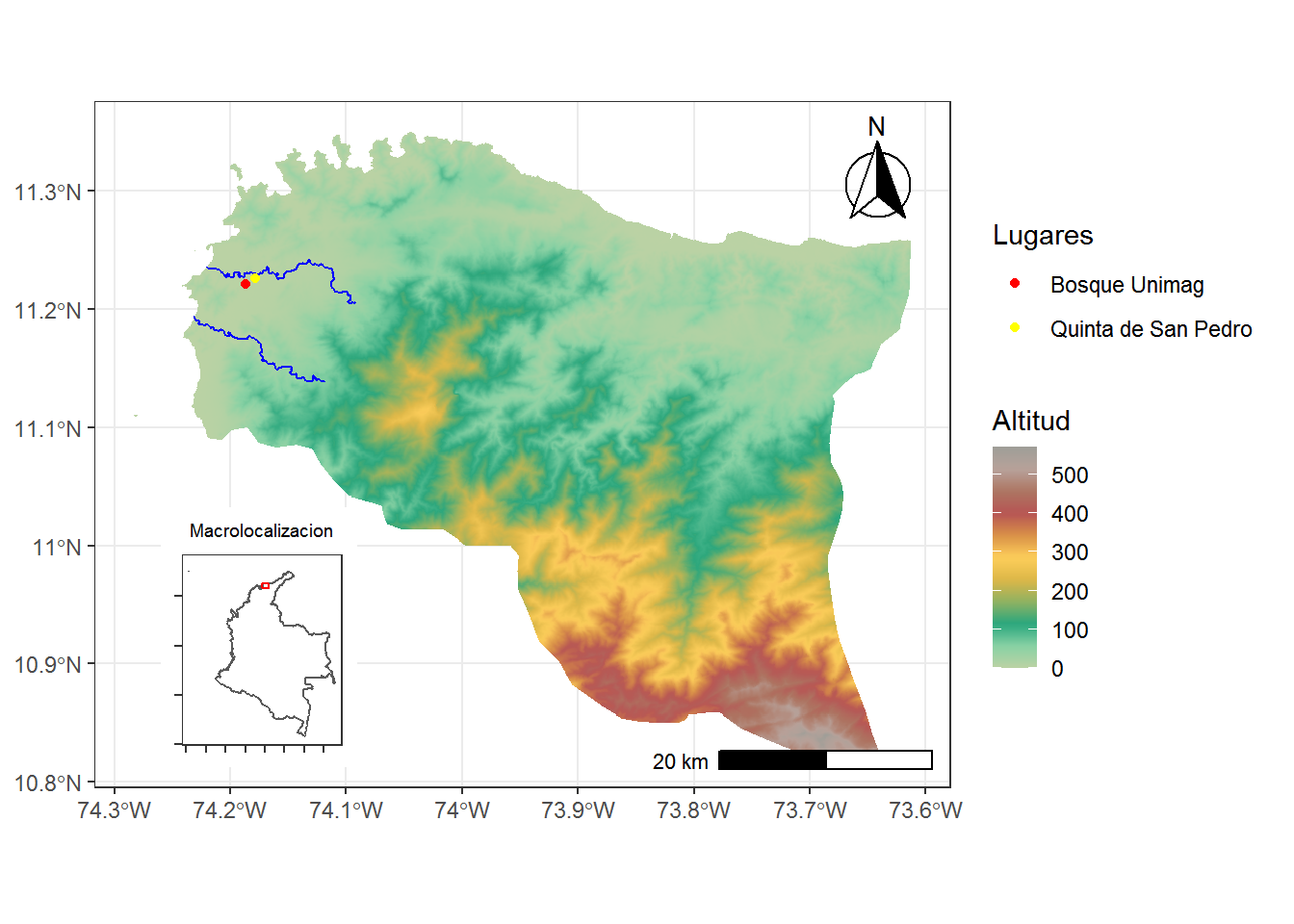

13. guardar el mapa

#ggsave(plot = mapa_final, filename = './mapa_final.png', dpi = 300)

14. Interactivo

tmap::tmap_mode("view")

## tmap mode set to interactive viewing

tmap::tm_shape(lugar) + tm_bubbles(size = 2, col = "red")